Active learning for 2D classification
In this tutorial, we showcase active learning using the posterior uncertainty on a two-dimensional classification task with three classes. The tutorial relies on concepts from the tutorial for active learning on regression.
from functools import partial

import jax
import optax
from flax import nnx
from helper import DataLoader, Model, split, train_model
from jax import numpy as jnp
from jax import random
from matplotlib import pyplot as plt
from optax.losses import softmax_cross_entropy_with_integer_labels
from plotting import (
    plot_datapoints,
    plot_decision_boundaries,
    plot_next_point,
    plot_prediction,
    show_animation_classification,
)
from tqdm import tqdm

from laplax.api import calibration, estimate_curvature
from laplax.curv import create_ggn_mv, create_posterior_fn
from laplax.eval.pushforward import (
    lin_pred_mean,
    lin_pred_std,
    lin_setup,
    set_lin_pushforward,
)

seed = 2392386
key = random.key(seed)
init_data_key, cali_data_key, passive_data_key, sampling_key = random.split(key, 4)
First, we define the ground truth decision boundary function.
@jax.jit
def true_function(point):
    def f1(x):
        return 1.9 * x**3 - 1.5 * x**2 + 0.5

    def f2(x):
        return -1.5 * x**2 + 2 * x + 0.2

    x, y = point[0], point[1]
    return jnp.where(y >= f2(x), 2, jnp.where(y >= f1(x), 1, 0))
We generate some initial datapoints and visualize them.
n_initial_datapoints = 20


def generate_dataset(n_points, key):
    key1, key2 = random.split(key)
    xs = random.uniform(key1, shape=n_points, minval=0, maxval=1)
    ys = random.uniform(key2, shape=n_points, minval=0, maxval=1)
    datapoints = jnp.stack((xs, ys)).mT
    labels = jax.vmap(true_function)(datapoints)
    return DataLoader(datapoints, labels, batch_size=10)


class_dataloader = generate_dataset(n_initial_datapoints, init_data_key)
plt.figure(figsize=(5, 5))
plot_decision_boundaries()
plot_datapoints(class_dataloader)
plt.show()
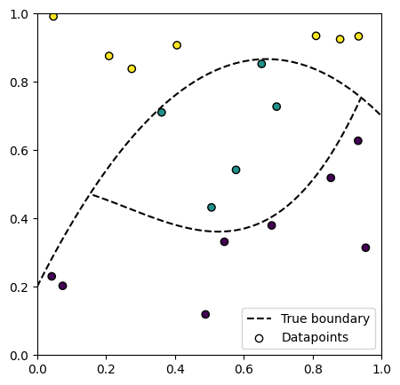
As our model, we reuse the model from the other active learning tutorial, a small fully connected network with four layers. Here, we have 2 input features, 3 output logits and use cross entropy loss.
We train the model on a small starting batch of datapoints.
@nnx.jit
def train_step(model, optimizer, batch, labels):
    def loss_fn(model):
        logits = model(batch)
        return softmax_cross_entropy_with_integer_labels(logits, labels).sum()

    loss, grads = nnx.value_and_grad(loss_fn)(model)
    optimizer.update(grads)
    return loss


start_model = Model(
    in_channels=2, hidden_channels=32, out_channels=3, rngs=nnx.Rngs(seed)
)

params = nnx.state(start_model)
total_params = sum(p.size for p in jax.tree.leaves(params))
print(f"Total number of parameters: {total_params}")

lr = 1e-3
n_initial_epochs = n_initial_datapoints * 50
class_optimizer = nnx.Optimizer(start_model, optax.adam(lr))
class_model = train_model(
    start_model,
    class_optimizer,
    class_dataloader,
    train_step,
    n_epochs=n_initial_epochs,
)
Total number of parameters: 2307


[epoch 100]: loss: 3.9805


[epoch 200]: loss: 2.5013


[epoch 300]: loss: 1.6488


[epoch 400]: loss: 0.5547


[epoch 500]: loss: 0.2016


[epoch 600]: loss: 0.1118


[epoch 700]: loss: 0.0447


[epoch 800]: loss: 0.0324


[epoch 900]: loss: 0.0296


Final loss: 0.0138
We visualize the trained model's predictions as background color in the data plane.
xv, yv = jnp.meshgrid(jnp.linspace(0, 1, 100), jnp.linspace(0, 1, 100))
gridpoints = jnp.stack([xv.ravel(), yv.ravel()], axis=-1)
true_labels = jax.vmap(true_function)(gridpoints)
logits = jax.vmap(class_model)(gridpoints)
preds = logits.argmax(axis=-1)

plot_decision_boundaries()
plot_datapoints(class_dataloader)
plot_prediction(preds)
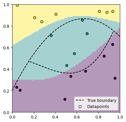
The existent data is fit well, indicating that the training has worked. The true decision boundary is not recovered however, simply because the model hasn't seen enough data yet. We are going to continue learning with more actively chosen data.
In this example, we use the first rule for maximal total information gain, as shown in the active learning tutorial for regression. The maximum of the total information gain is at the same location as the maximum of the model's predicted standard deviation, as the constants and logarithm in the formula do not change the location of the maximum. Therefore, it is sufficient here to calculate the posterior uncertainty using laplax. As in the other tutorial, we calibrate the prior precision to get meaningful uncertainty estimates. This time however, we calibrate on a calibration dataset. This is because on the training dataset, the model makes no errors and hence, the calibrated prior precision diverges to large values. This leads to bad results during active learning. Of course, this introduces a dependency on more datapoints compared to passive learning, which does not align well with the goal to make learning more data-efficient. We argue however that a validation set is anyway needed to optimize other hyperparameters in a realistic setting, and that the prior precision is just another hyperparameter to be fitted using this validation set.
def construct_prob_predictive(data, model):
    dataset = {"input": data.X, "target": data.y}
    model_fn, params = split(model)
    ggn_mv = create_ggn_mv(
        model_fn,
        params,
        dataset,
        loss_fn="cross_entropy",
    )
    posterior_fn = create_posterior_fn(
        curv_type="full",
        mv=ggn_mv,
        layout=params,
    )
    prob_predictive = partial(
        set_lin_pushforward,
        model_fn=model_fn,
        mean_params=params,
        posterior_fn=posterior_fn,
        pushforward_fns=[
            lin_setup,
            lin_pred_mean,
            lin_pred_std,
        ],
    )
    return dataset, model_fn, params, ggn_mv, posterior_fn, prob_predictive


def calibrate_prior_precision(data, model, grid_params):
    """Calibrate the prior precision.

    Args:
        data: dataloader to use for calibration
        model: nnx.Module
        grid_params: dict of parameters for grid search

    Returns:
        Calibrated prior precision.
    """
    dataset, model_fn, params, ggn_mv, posterior_fn, _ = construct_prob_predictive(
        data, model
    )
    curv_estimate = estimate_curvature(
        curv_type="full",
        mv=ggn_mv,
        layout=params,
    )
    return calibration(
        posterior_fn=posterior_fn,
        model_fn=model_fn,
        params=params,
        data=dataset,
        loss_fn="CROSS_ENTROPY",
        predictive_type="MC_BRIDGE",
        curv_estimate=curv_estimate,
        curv_type="full",
        calibration_objective="ECE",
        calibration_method="GRID_SEARCH",
        **grid_params,
    )[0]


grid_params = {
    "log_prior_prec_min": -2.0,
    "log_prior_prec_max": 3.0,
    "grid_size": 100,
}

n_calibration_datapoints = 30
cali_dataloader = generate_dataset(n_calibration_datapoints, cali_data_key)

prior_args = calibrate_prior_precision(cali_dataloader, class_model, grid_params)


print("Prior precision: ", prior_args["prior_prec"])
[32m2026-06-16 09:39:38.636[0m | [34m[1mDEBUG [0m | [36mlaplax.api[0m:[36mcalibration[0m:[36m828[0m - [34m[1mStarting calibration with objective ECE on grid [-2.0, 3.0] (100 pts, pat=None)[0m
[32m2026-06-16 09:39:40.304[0m | [1mINFO [0m | [36mlaplax.eval.calibrate[0m:[36mgrid_search[0m:[36m110[0m - [1mTook 1.5119 seconds, prior prec: 0.0100, result: 0.364996[0m
[32m2026-06-16 09:39:40.462[0m | [1mINFO [0m | [36mlaplax.eval.calibrate[0m:[36mgrid_search[0m:[36m110[0m - [1mTook 0.1548 seconds, prior prec: 0.0112, result: 0.359458[0m
[32m2026-06-16 09:39:40.617[0m | [1mINFO [0m | [36mlaplax.eval.calibrate[0m:[36mgrid_search[0m:[36m110[0m - [1mTook 0.1544 seconds, prior prec: 0.0126, result: 0.354498[0m
[32m2026-06-16 09:39:40.769[0m | [1mINFO [0m | [36mlaplax.eval.calibrate[0m:[36mgrid_search[0m:[36m110[0m - [1mTook 0.1513 seconds, prior prec: 0.0142, result: 0.350011[0m
[32m2026-06-16 09:39:40.923[0m | [1mINFO [0m | [36mlaplax.eval.calibrate[0m:[36mgrid_search[0m:[36m110[0m - [1mTook 0.1527 seconds, prior prec: 0.0159, result: 0.346636[0m
[32m2026-06-16 09:39:41.079[0m | [1mINFO [0m | [36mlaplax.eval.calibrate[0m:[36mgrid_search[0m:[36m110[0m - [1mTook 0.1541 seconds, prior prec: 0.0179, result: 0.342523[0m
[32m2026-06-16 09:39:41.238[0m | [1mINFO [0m | [36mlaplax.eval.calibrate[0m:[36mgrid_search[0m:[36m110[0m - [1mTook 0.1564 seconds, prior prec: 0.0201, result: 0.338403[0m
[32m2026-06-16 09:39:41.393[0m | [1mINFO [0m | [36mlaplax.eval.calibrate[0m:[36mgrid_search[0m:[36m110[0m - [1mTook 0.1525 seconds, prior prec: 0.0226, result: 0.334142[0m
[32m2026-06-16 09:39:41.547[0m | [1mINFO [0m | [36mlaplax.eval.calibrate[0m:[36mgrid_search[0m:[36m110[0m - [1mTook 0.1534 seconds, prior prec: 0.0254, result: 0.329128[0m
[32m2026-06-16 09:39:41.696[0m | [1mINFO [0m | [36mlaplax.eval.calibrate[0m:[36mgrid_search[0m:[36m110[0m - [1mTook 0.1482 seconds, prior prec: 0.0285, result: 0.324095[0m
[32m2026-06-16 09:39:41.850[0m | [1mINFO [0m | [36mlaplax.eval.calibrate[0m:[36mgrid_search[0m:[36m110[0m - [1mTook 0.1532 seconds, prior prec: 0.0320, result: 0.318212[0m
[32m2026-06-16 09:39:42.003[0m | [1mINFO [0m | [36mlaplax.eval.calibrate[0m:[36mgrid_search[0m:[36m110[0m - [1mTook 0.1503 seconds, prior prec: 0.0359, result: 0.315242[0m
[32m2026-06-16 09:39:42.159[0m | [1mINFO [0m | [36mlaplax.eval.calibrate[0m:[36mgrid_search[0m:[36m110[0m - [1mTook 0.1552 seconds, prior prec: 0.0404, result: 0.319564[0m
[32m2026-06-16 09:39:42.316[0m | [1mINFO [0m | [36mlaplax.eval.calibrate[0m:[36mgrid_search[0m:[36m110[0m - [1mTook 0.1548 seconds, prior prec: 0.0453, result: 0.317366[0m
[32m2026-06-16 09:39:42.467[0m | [1mINFO [0m | [36mlaplax.eval.calibrate[0m:[36mgrid_search[0m:[36m110[0m - [1mTook 0.1498 seconds, prior prec: 0.0509, result: 0.319219[0m
[32m2026-06-16 09:39:42.620[0m | [1mINFO [0m | [36mlaplax.eval.calibrate[0m:[36mgrid_search[0m:[36m110[0m - [1mTook 0.1525 seconds, prior prec: 0.0572, result: 0.340520[0m
[32m2026-06-16 09:39:42.777[0m | [1mINFO [0m | [36mlaplax.eval.calibrate[0m:[36mgrid_search[0m:[36m110[0m - [1mTook 0.1555 seconds, prior prec: 0.0643, result: 0.334906[0m
[32m2026-06-16 09:39:42.937[0m | [1mINFO [0m | [36mlaplax.eval.calibrate[0m:[36mgrid_search[0m:[36m110[0m - [1mTook 0.1579 seconds, prior prec: 0.0722, result: 0.334296[0m
[32m2026-06-16 09:39:43.095[0m | [1mINFO [0m | [36mlaplax.eval.calibrate[0m:[36mgrid_search[0m:[36m110[0m - [1mTook 0.1567 seconds, prior prec: 0.0811, result: 0.288514[0m
[32m2026-06-16 09:39:43.250[0m | [1mINFO [0m | [36mlaplax.eval.calibrate[0m:[36mgrid_search[0m:[36m110[0m - [1mTook 0.1543 seconds, prior prec: 0.0911, result: 0.272358[0m
[32m2026-06-16 09:39:43.404[0m | [1mINFO [0m | [36mlaplax.eval.calibrate[0m:[36mgrid_search[0m:[36m110[0m - [1mTook 0.1537 seconds, prior prec: 0.1024, result: 0.261697[0m
[32m2026-06-16 09:39:43.561[0m | [1mINFO [0m | [36mlaplax.eval.calibrate[0m:[36mgrid_search[0m:[36m110[0m - [1mTook 0.1555 seconds, prior prec: 0.1150, result: 0.268431[0m
[32m2026-06-16 09:39:43.718[0m | [1mINFO [0m | [36mlaplax.eval.calibrate[0m:[36mgrid_search[0m:[36m110[0m - [1mTook 0.1560 seconds, prior prec: 0.1292, result: 0.297118[0m
[32m2026-06-16 09:39:43.873[0m | [1mINFO [0m | [36mlaplax.eval.calibrate[0m:[36mgrid_search[0m:[36m110[0m - [1mTook 0.1546 seconds, prior prec: 0.1451, result: 0.260267[0m
[32m2026-06-16 09:39:44.029[0m | [1mINFO [0m | [36mlaplax.eval.calibrate[0m:[36mgrid_search[0m:[36m110[0m - [1mTook 0.1550 seconds, prior prec: 0.1630, result: 0.211198[0m
[32m2026-06-16 09:39:44.187[0m | [1mINFO [0m | [36mlaplax.eval.calibrate[0m:[36mgrid_search[0m:[36m110[0m - [1mTook 0.1567 seconds, prior prec: 0.1831, result: 0.268678[0m
[32m2026-06-16 09:39:44.340[0m | [1mINFO [0m | [36mlaplax.eval.calibrate[0m:[36mgrid_search[0m:[36m110[0m - [1mTook 0.1523 seconds, prior prec: 0.2057, result: 0.237320[0m
[32m2026-06-16 09:39:44.493[0m | [1mINFO [0m | [36mlaplax.eval.calibrate[0m:[36mgrid_search[0m:[36m110[0m - [1mTook 0.1521 seconds, prior prec: 0.2310, result: 0.245382[0m
[32m2026-06-16 09:39:44.649[0m | [1mINFO [0m | [36mlaplax.eval.calibrate[0m:[36mgrid_search[0m:[36m110[0m - [1mTook 0.1543 seconds, prior prec: 0.2595, result: 0.201112[0m
[32m2026-06-16 09:39:44.803[0m | [1mINFO [0m | [36mlaplax.eval.calibrate[0m:[36mgrid_search[0m:[36m110[0m - [1mTook 0.1528 seconds, prior prec: 0.2915, result: 0.198170[0m
[32m2026-06-16 09:39:44.960[0m | [1mINFO [0m | [36mlaplax.eval.calibrate[0m:[36mgrid_search[0m:[36m110[0m - [1mTook 0.1562 seconds, prior prec: 0.3275, result: 0.148281[0m
[32m2026-06-16 09:39:45.113[0m | [1mINFO [0m | [36mlaplax.eval.calibrate[0m:[36mgrid_search[0m:[36m110[0m - [1mTook 0.1522 seconds, prior prec: 0.3678, result: 0.123452[0m
[32m2026-06-16 09:39:45.268[0m | [1mINFO [0m | [36mlaplax.eval.calibrate[0m:[36mgrid_search[0m:[36m110[0m - [1mTook 0.1529 seconds, prior prec: 0.4132, result: 0.101501[0m
[32m2026-06-16 09:39:45.424[0m | [1mINFO [0m | [36mlaplax.eval.calibrate[0m:[36mgrid_search[0m:[36m110[0m - [1mTook 0.1541 seconds, prior prec: 0.4642, result: 0.158843[0m
[32m2026-06-16 09:39:45.582[0m | [1mINFO [0m | [36mlaplax.eval.calibrate[0m:[36mgrid_search[0m:[36m110[0m - [1mTook 0.1573 seconds, prior prec: 0.5214, result: 0.126424[0m
[32m2026-06-16 09:39:45.740[0m | [1mINFO [0m | [36mlaplax.eval.calibrate[0m:[36mgrid_search[0m:[36m110[0m - [1mTook 0.1565 seconds, prior prec: 0.5857, result: 0.117565[0m
[32m2026-06-16 09:39:45.898[0m | [1mINFO [0m | [36mlaplax.eval.calibrate[0m:[36mgrid_search[0m:[36m110[0m - [1mTook 0.1567 seconds, prior prec: 0.6579, result: 0.177935[0m
[32m2026-06-16 09:39:46.046[0m | [1mINFO [0m | [36mlaplax.eval.calibrate[0m:[36mgrid_search[0m:[36m110[0m - [1mTook 0.1474 seconds, prior prec: 0.7391, result: 0.177305[0m
[32m2026-06-16 09:39:46.189[0m | [1mINFO [0m | [36mlaplax.eval.calibrate[0m:[36mgrid_search[0m:[36m110[0m - [1mTook 0.1421 seconds, prior prec: 0.8302, result: 0.183047[0m
[32m2026-06-16 09:39:46.340[0m | [1mINFO [0m | [36mlaplax.eval.calibrate[0m:[36mgrid_search[0m:[36m110[0m - [1mTook 0.1492 seconds, prior prec: 0.9326, result: 0.127367[0m
[32m2026-06-16 09:39:46.499[0m | [1mINFO [0m | [36mlaplax.eval.calibrate[0m:[36mgrid_search[0m:[36m110[0m - [1mTook 0.1577 seconds, prior prec: 1.0476, result: 0.134838[0m
[32m2026-06-16 09:39:46.657[0m | [1mINFO [0m | [36mlaplax.eval.calibrate[0m:[36mgrid_search[0m:[36m110[0m - [1mTook 0.1563 seconds, prior prec: 1.1768, result: 0.156459[0m
[32m2026-06-16 09:39:46.815[0m | [1mINFO [0m | [36mlaplax.eval.calibrate[0m:[36mgrid_search[0m:[36m110[0m - [1mTook 0.1573 seconds, prior prec: 1.3219, result: 0.203297[0m
[32m2026-06-16 09:39:46.971[0m | [1mINFO [0m | [36mlaplax.eval.calibrate[0m:[36mgrid_search[0m:[36m110[0m - [1mTook 0.1540 seconds, prior prec: 1.4850, result: 0.201936[0m
[32m2026-06-16 09:39:47.125[0m | [1mINFO [0m | [36mlaplax.eval.calibrate[0m:[36mgrid_search[0m:[36m110[0m - [1mTook 0.1538 seconds, prior prec: 1.6681, result: 0.179132[0m
[32m2026-06-16 09:39:47.276[0m | [1mINFO [0m | [36mlaplax.eval.calibrate[0m:[36mgrid_search[0m:[36m110[0m - [1mTook 0.1487 seconds, prior prec: 1.8738, result: 0.185622[0m
[32m2026-06-16 09:39:47.456[0m | [1mINFO [0m | [36mlaplax.eval.calibrate[0m:[36mgrid_search[0m:[36m110[0m - [1mTook 0.1788 seconds, prior prec: 2.1049, result: 0.165907[0m
[32m2026-06-16 09:39:47.612[0m | [1mINFO [0m | [36mlaplax.eval.calibrate[0m:[36mgrid_search[0m:[36m110[0m - [1mTook 0.1553 seconds, prior prec: 2.3645, result: 0.147422[0m
[32m2026-06-16 09:39:47.757[0m | [1mINFO [0m | [36mlaplax.eval.calibrate[0m:[36mgrid_search[0m:[36m110[0m - [1mTook 0.1447 seconds, prior prec: 2.6561, result: 0.151018[0m
[32m2026-06-16 09:39:47.937[0m | [1mINFO [0m | [36mlaplax.eval.calibrate[0m:[36mgrid_search[0m:[36m110[0m - [1mTook 0.1780 seconds, prior prec: 2.9836, result: 0.162416[0m
[32m2026-06-16 09:39:48.091[0m | [1mINFO [0m | [36mlaplax.eval.calibrate[0m:[36mgrid_search[0m:[36m110[0m - [1mTook 0.1531 seconds, prior prec: 3.3516, result: 0.107684[0m
[32m2026-06-16 09:39:48.249[0m | [1mINFO [0m | [36mlaplax.eval.calibrate[0m:[36mgrid_search[0m:[36m110[0m - [1mTook 0.1567 seconds, prior prec: 3.7649, result: 0.111784[0m
[32m2026-06-16 09:39:48.402[0m | [1mINFO [0m | [36mlaplax.eval.calibrate[0m:[36mgrid_search[0m:[36m110[0m - [1mTook 0.1513 seconds, prior prec: 4.2292, result: 0.115569[0m
[32m2026-06-16 09:39:48.559[0m | [1mINFO [0m | [36mlaplax.eval.calibrate[0m:[36mgrid_search[0m:[36m110[0m - [1mTook 0.1556 seconds, prior prec: 4.7508, result: 0.119100[0m
[32m2026-06-16 09:39:48.713[0m | [1mINFO [0m | [36mlaplax.eval.calibrate[0m:[36mgrid_search[0m:[36m110[0m - [1mTook 0.1522 seconds, prior prec: 5.3367, result: 0.122435[0m
[32m2026-06-16 09:39:48.868[0m | [1mINFO [0m | [36mlaplax.eval.calibrate[0m:[36mgrid_search[0m:[36m110[0m - [1mTook 0.1527 seconds, prior prec: 5.9948, result: 0.125640[0m
[32m2026-06-16 09:39:49.023[0m | [1mINFO [0m | [36mlaplax.eval.calibrate[0m:[36mgrid_search[0m:[36m110[0m - [1mTook 0.1541 seconds, prior prec: 6.7342, result: 0.128752[0m
[32m2026-06-16 09:39:49.175[0m | [1mINFO [0m | [36mlaplax.eval.calibrate[0m:[36mgrid_search[0m:[36m110[0m - [1mTook 0.1514 seconds, prior prec: 7.5646, result: 0.149807[0m
[32m2026-06-16 09:39:49.331[0m | [1mINFO [0m | [36mlaplax.eval.calibrate[0m:[36mgrid_search[0m:[36m110[0m - [1mTook 0.1548 seconds, prior prec: 8.4975, result: 0.159940[0m
[32m2026-06-16 09:39:49.488[0m | [1mINFO [0m | [36mlaplax.eval.calibrate[0m:[36mgrid_search[0m:[36m110[0m - [1mTook 0.1563 seconds, prior prec: 9.5455, result: 0.168950[0m
[32m2026-06-16 09:39:49.643[0m | [1mINFO [0m | [36mlaplax.eval.calibrate[0m:[36mgrid_search[0m:[36m110[0m - [1mTook 0.1532 seconds, prior prec: 10.7227, result: 0.164738[0m
[32m2026-06-16 09:39:49.794[0m | [1mINFO [0m | [36mlaplax.eval.calibrate[0m:[36mgrid_search[0m:[36m110[0m - [1mTook 0.1503 seconds, prior prec: 12.0450, result: 0.165597[0m
[32m2026-06-16 09:39:49.952[0m | [1mINFO [0m | [36mlaplax.eval.calibrate[0m:[36mgrid_search[0m:[36m110[0m - [1mTook 0.1568 seconds, prior prec: 13.5305, result: 0.166411[0m
[32m2026-06-16 09:39:50.105[0m | [1mINFO [0m | [36mlaplax.eval.calibrate[0m:[36mgrid_search[0m:[36m110[0m - [1mTook 0.1524 seconds, prior prec: 15.1991, result: 0.146216[0m
[32m2026-06-16 09:39:50.262[0m | [1mINFO [0m | [36mlaplax.eval.calibrate[0m:[36mgrid_search[0m:[36m110[0m - [1mTook 0.1546 seconds, prior prec: 17.0735, result: 0.148079[0m
[32m2026-06-16 09:39:50.429[0m | [1mINFO [0m | [36mlaplax.eval.calibrate[0m:[36mgrid_search[0m:[36m110[0m - [1mTook 0.1650 seconds, prior prec: 19.1791, result: 0.149798[0m
[32m2026-06-16 09:39:50.587[0m | [1mINFO [0m | [36mlaplax.eval.calibrate[0m:[36mgrid_search[0m:[36m110[0m - [1mTook 0.1576 seconds, prior prec: 21.5443, result: 0.151352[0m
[32m2026-06-16 09:39:50.740[0m | [1mINFO [0m | [36mlaplax.eval.calibrate[0m:[36mgrid_search[0m:[36m110[0m - [1mTook 0.1516 seconds, prior prec: 24.2013, result: 0.164361[0m
[32m2026-06-16 09:39:50.898[0m | [1mINFO [0m | [36mlaplax.eval.calibrate[0m:[36mgrid_search[0m:[36m110[0m - [1mTook 0.1568 seconds, prior prec: 27.1859, result: 0.165400[0m
[32m2026-06-16 09:39:51.055[0m | [1mINFO [0m | [36mlaplax.eval.calibrate[0m:[36mgrid_search[0m:[36m110[0m - [1mTook 0.1554 seconds, prior prec: 30.5386, result: 0.166274[0m
[32m2026-06-16 09:39:51.238[0m | [1mINFO [0m | [36mlaplax.eval.calibrate[0m:[36mgrid_search[0m:[36m110[0m - [1mTook 0.1821 seconds, prior prec: 34.3047, result: 0.167000[0m
[32m2026-06-16 09:39:51.388[0m | [1mINFO [0m | [36mlaplax.eval.calibrate[0m:[36mgrid_search[0m:[36m110[0m - [1mTook 0.1488 seconds, prior prec: 38.5353, result: 0.167600[0m
[32m2026-06-16 09:39:51.542[0m | [1mINFO [0m | [36mlaplax.eval.calibrate[0m:[36mgrid_search[0m:[36m110[0m - [1mTook 0.1530 seconds, prior prec: 43.2876, result: 0.168089[0m
[32m2026-06-16 09:39:51.693[0m | [1mINFO [0m | [36mlaplax.eval.calibrate[0m:[36mgrid_search[0m:[36m110[0m - [1mTook 0.1508 seconds, prior prec: 48.6260, result: 0.168483[0m
[32m2026-06-16 09:39:51.840[0m | [1mINFO [0m | [36mlaplax.eval.calibrate[0m:[36mgrid_search[0m:[36m110[0m - [1mTook 0.1447 seconds, prior prec: 54.6228, result: 0.168792[0m
[32m2026-06-16 09:39:51.989[0m | [1mINFO [0m | [36mlaplax.eval.calibrate[0m:[36mgrid_search[0m:[36m110[0m - [1mTook 0.1469 seconds, prior prec: 61.3591, result: 0.169027[0m
[32m2026-06-16 09:39:52.141[0m | [1mINFO [0m | [36mlaplax.eval.calibrate[0m:[36mgrid_search[0m:[36m110[0m - [1mTook 0.1510 seconds, prior prec: 68.9262, result: 0.151820[0m
[32m2026-06-16 09:39:52.294[0m | [1mINFO [0m | [36mlaplax.eval.calibrate[0m:[36mgrid_search[0m:[36m110[0m - [1mTook 0.1513 seconds, prior prec: 77.4264, result: 0.152363[0m
[32m2026-06-16 09:39:52.451[0m | [1mINFO [0m | [36mlaplax.eval.calibrate[0m:[36mgrid_search[0m:[36m110[0m - [1mTook 0.1563 seconds, prior prec: 86.9749, result: 0.152873[0m
[32m2026-06-16 09:39:52.606[0m | [1mINFO [0m | [36mlaplax.eval.calibrate[0m:[36mgrid_search[0m:[36m110[0m - [1mTook 0.1546 seconds, prior prec: 97.7010, result: 0.153353[0m
[32m2026-06-16 09:39:52.761[0m | [1mINFO [0m | [36mlaplax.eval.calibrate[0m:[36mgrid_search[0m:[36m110[0m - [1mTook 0.1523 seconds, prior prec: 109.7499, result: 0.153809[0m
[32m2026-06-16 09:39:52.911[0m | [1mINFO [0m | [36mlaplax.eval.calibrate[0m:[36mgrid_search[0m:[36m110[0m - [1mTook 0.1477 seconds, prior prec: 123.2847, result: 0.154240[0m
[32m2026-06-16 09:39:53.069[0m | [1mINFO [0m | [36mlaplax.eval.calibrate[0m:[36mgrid_search[0m:[36m110[0m - [1mTook 0.1564 seconds, prior prec: 138.4886, result: 0.137335[0m
[32m2026-06-16 09:39:53.224[0m | [1mINFO [0m | [36mlaplax.eval.calibrate[0m:[36mgrid_search[0m:[36m110[0m - [1mTook 0.1547 seconds, prior prec: 155.5676, result: 0.143454[0m
[32m2026-06-16 09:39:53.379[0m | [1mINFO [0m | [36mlaplax.eval.calibrate[0m:[36mgrid_search[0m:[36m110[0m - [1mTook 0.1534 seconds, prior prec: 174.7528, result: 0.144328[0m
[32m2026-06-16 09:39:53.533[0m | [1mINFO [0m | [36mlaplax.eval.calibrate[0m:[36mgrid_search[0m:[36m110[0m - [1mTook 0.1530 seconds, prior prec: 196.3041, result: 0.158184[0m
[32m2026-06-16 09:39:53.687[0m | [1mINFO [0m | [36mlaplax.eval.calibrate[0m:[36mgrid_search[0m:[36m110[0m - [1mTook 0.1536 seconds, prior prec: 220.5132, result: 0.158572[0m
[32m2026-06-16 09:39:53.842[0m | [1mINFO [0m | [36mlaplax.eval.calibrate[0m:[36mgrid_search[0m:[36m110[0m - [1mTook 0.1537 seconds, prior prec: 247.7077, result: 0.154559[0m
[32m2026-06-16 09:39:53.995[0m | [1mINFO [0m | [36mlaplax.eval.calibrate[0m:[36mgrid_search[0m:[36m110[0m - [1mTook 0.1524 seconds, prior prec: 278.2559, result: 0.168163[0m
[32m2026-06-16 09:39:54.154[0m | [1mINFO [0m | [36mlaplax.eval.calibrate[0m:[36mgrid_search[0m:[36m110[0m - [1mTook 0.1568 seconds, prior prec: 312.5717, result: 0.167975[0m
[32m2026-06-16 09:39:54.308[0m | [1mINFO [0m | [36mlaplax.eval.calibrate[0m:[36mgrid_search[0m:[36m110[0m - [1mTook 0.1518 seconds, prior prec: 351.1191, result: 0.167784[0m
[32m2026-06-16 09:39:54.466[0m | [1mINFO [0m | [36mlaplax.eval.calibrate[0m:[36mgrid_search[0m:[36m110[0m - [1mTook 0.1562 seconds, prior prec: 394.4207, result: 0.146302[0m
[32m2026-06-16 09:39:54.620[0m | [1mINFO [0m | [36mlaplax.eval.calibrate[0m:[36mgrid_search[0m:[36m110[0m - [1mTook 0.1530 seconds, prior prec: 443.0623, result: 0.147183[0m
[32m2026-06-16 09:39:54.777[0m | [1mINFO [0m | [36mlaplax.eval.calibrate[0m:[36mgrid_search[0m:[36m110[0m - [1mTook 0.1549 seconds, prior prec: 497.7027, result: 0.148034[0m
[32m2026-06-16 09:39:54.927[0m | [1mINFO [0m | [36mlaplax.eval.calibrate[0m:[36mgrid_search[0m:[36m110[0m - [1mTook 0.1497 seconds, prior prec: 559.0812, result: 0.148856[0m
[32m2026-06-16 09:39:55.083[0m | [1mINFO [0m | [36mlaplax.eval.calibrate[0m:[36mgrid_search[0m:[36m110[0m - [1mTook 0.1543 seconds, prior prec: 628.0292, result: 0.166871[0m
[32m2026-06-16 09:39:55.237[0m | [1mINFO [0m | [36mlaplax.eval.calibrate[0m:[36mgrid_search[0m:[36m110[0m - [1mTook 0.1534 seconds, prior prec: 705.4805, result: 0.166716[0m
[32m2026-06-16 09:39:55.396[0m | [1mINFO [0m | [36mlaplax.eval.calibrate[0m:[36mgrid_search[0m:[36m110[0m - [1mTook 0.1569 seconds, prior prec: 792.4829, result: 0.166578[0m
[32m2026-06-16 09:39:55.552[0m | [1mINFO [0m | [36mlaplax.eval.calibrate[0m:[36mgrid_search[0m:[36m110[0m - [1mTook 0.1541 seconds, prior prec: 890.2148, result: 0.166456[0m
[32m2026-06-16 09:39:55.706[0m | [1mINFO [0m | [36mlaplax.eval.calibrate[0m:[36mgrid_search[0m:[36m110[0m - [1mTook 0.1532 seconds, prior prec: 1000.0000, result: 0.166354[0m
[32m2026-06-16 09:39:55.708[0m | [1mINFO [0m | [36mlaplax.eval.calibrate[0m:[36mgrid_search[0m:[36m139[0m - [1mChosen prior prec = 0.4132[0m
[32m2026-06-16 09:39:55.772[0m | [34m[1mDEBUG [0m | [36mlaplax.api[0m:[36mcalibration[0m:[36m866[0m - [34m[1mCalibrated prior args = {'prior_prec': Array(0.4132012, dtype=float32)}[0m
Prior precision: 0.4132012
def compute_uncertainty(prob_predictive, prior_args):
    prob_predictive = prob_predictive(prior_arguments=prior_args)
    pred = jax.vmap(prob_predictive)(gridpoints)
    return pred["pred_std"]


prob_predictive = construct_prob_predictive(class_dataloader, class_model)[-1]
uncertainties = compute_uncertainty(prob_predictive, prior_args)
uncertainty = uncertainties[jnp.arange(10000), preds]
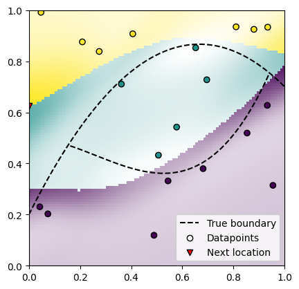
We calculate the uncertainty on a regular grid within data space, and find its maximum on the grid. This is going to be the best next datapoint location. We visualize the uncertainty as the alpha-value of the prediction colors, with stronger color corresponding to larger uncertainty.
'get_next_point_sampled' is an alternative rule to find the next datapoint, which samples from the data plane by interpreting the uncertainty as logits to a categorical distribution. This way, random points with high uncertainty are chosen, which prevents the active learning loop from sampling in the same region repeatedly. Feel free to try out both methods in the active learning loop and see the difference!
def get_next_point(uncertainty):
    return gridpoints[jnp.argmax(uncertainty)]


def get_next_point_sampled(key, uncertainty):
    return gridpoints[jax.random.categorical(key, uncertainty)]


next_point = get_next_point(uncertainty)

plot_decision_boundaries()
plot_datapoints(class_dataloader)
plot_prediction(preds, uncertainty)
plot_next_point(next_point)
def evaluate(model):
    logits = jax.vmap(model)(gridpoints)
    preds = logits.argmax(axis=-1)
    return preds


def accuracy(model):
    preds = evaluate(model)
    acc = jnp.mean(preds == true_labels)
    return acc
We see that the uncertainty is large where the model thinks the decision boundary lies, and low elsewhere. This means the active learning loop, which we are going to implement next, is going to sample in these areas, confirming or adapting the found decision boundary.
learning_rounds = 50
epochs_per_learning_round = 35
plot_data = []
sampling_keys = jax.random.split(sampling_key, learning_rounds)
accuracies = []

# To keep the rendered output readable, we only print the details of the first
# `verbose_rounds` rounds (raise this to see more).
verbose_rounds = 2

for i, _key in tqdm(enumerate(sampling_keys)):
    verbose = i < verbose_rounds
    if verbose:
        print(f"Active learning round {i + 1}")
    # 1) Sample new datapoint
    next_target = true_function(next_point)
    class_dataloader = class_dataloader.add(next_point, jnp.atleast_1d(next_target))

    # 2) Continue training
    class_model = train_model(
        class_model,
        class_optimizer,
        class_dataloader,
        train_step,
        n_epochs=epochs_per_learning_round,
        verbose=verbose,
    )
    grid_preds = jnp.argmax(class_model(gridpoints), axis=-1)

    # 3) Compute uncertainty
    prob_predictive = construct_prob_predictive(class_dataloader, class_model)[-1]
    uncertainties = compute_uncertainty(prob_predictive, prior_args)
    uncertainty = uncertainties[jnp.arange(10000), grid_preds]

    # 4) Find next datapoint location
    # next_point = get_next_point_sampled(_key, uncertainty)
    next_point = get_next_point(uncertainty)

    # Evaluation
    accuracies.append(accuracy(class_model))

    # Plotting
    data_preds = jnp.argmax(class_model(class_dataloader.X), axis=-1)
    plot_data.append((
        grid_preds,
        class_dataloader,
        uncertainty,
        next_point,
    ))
    if verbose:
        print("-----------------------")
    elif i == verbose_rounds:
        print(f"... (running {learning_rounds - verbose_rounds} more rounds) ...")
0it [00:00, ?it/s]
Active learning round 1


Final loss: 0.0000
1it [00:04, 4.48s/it]
-----------------------
Active learning round 2


Final loss: 0.0140
2it [00:08, 4.31s/it]
-----------------------
3it [00:13, 4.46s/it]
... (running 48 more rounds) ...
4it [00:18, 4.59s/it]
5it [00:22, 4.50s/it]
6it [00:26, 4.47s/it]
7it [00:31, 4.56s/it]
8it [00:35, 4.51s/it]
9it [00:40, 4.46s/it]
10it [00:44, 4.29s/it]
11it [00:48, 4.37s/it]
12it [00:52, 4.25s/it]
13it [00:57, 4.32s/it]
14it [01:01, 4.40s/it]
15it [01:05, 4.29s/it]
16it [01:10, 4.25s/it]
17it [01:14, 4.20s/it]
18it [01:18, 4.27s/it]
19it [01:22, 4.21s/it]
20it [01:26, 4.15s/it]
21it [01:30, 4.20s/it]
22it [01:35, 4.23s/it]
23it [01:39, 4.36s/it]
24it [01:43, 4.28s/it]
25it [01:48, 4.23s/it]
26it [01:52, 4.20s/it]
27it [01:56, 4.17s/it]
28it [02:00, 4.16s/it]
29it [02:04, 4.15s/it]
30it [02:08, 4.14s/it]
31it [02:12, 4.14s/it]
32it [02:17, 4.30s/it]
33it [02:21, 4.30s/it]
34it [02:25, 4.25s/it]
35it [02:30, 4.31s/it]
36it [02:34, 4.26s/it]
37it [02:38, 4.24s/it]
38it [02:42, 4.21s/it]
39it [02:47, 4.23s/it]
40it [02:51, 4.21s/it]
41it [02:55, 4.22s/it]
42it [03:00, 4.34s/it]
43it [03:04, 4.38s/it]
44it [03:09, 4.45s/it]
45it [03:13, 4.39s/it]
46it [03:18, 4.49s/it]
47it [03:22, 4.51s/it]
48it [03:27, 4.42s/it]
49it [03:31, 4.38s/it]
50it [03:35, 4.44s/it]
50it [03:35, 4.32s/it]
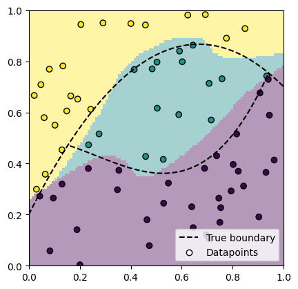
We see that the datapoints are concentrated around the true decision boundary, therefore increasing the gained information compared to sampling datapoints randomly from the plane.
Comparison against passive learning
As in the active learning example for regression, we compare our actively trained model against one that is trained as usual, with a fixed dataset.
n_passive_datapoints = n_initial_datapoints + learning_rounds
key1, key2 = random.split(passive_data_key)
xs = random.uniform(key1, shape=n_passive_datapoints, minval=0, maxval=1)
ys = random.uniform(key2, shape=n_passive_datapoints, minval=0, maxval=1)
datapoints = jnp.stack((xs, ys)).mT
labels = jax.vmap(true_function)(datapoints)
passive_class_dl = DataLoader(datapoints, labels, batch_size=10)

passive_class_model = Model(
    in_channels=2, hidden_channels=32, out_channels=3, rngs=nnx.Rngs(seed)
)
passive_class_optimizer = nnx.Optimizer(passive_class_model, optax.adam(lr))

n_epochs_passive = n_initial_epochs + learning_rounds * epochs_per_learning_round
passive_class_model = train_model(
    passive_class_model,
    passive_class_optimizer,
    passive_class_dl,
    train_step,
    n_epochs=n_epochs_passive,
)

passive_logits = jax.vmap(passive_class_model)(gridpoints)
passive_preds = passive_logits.argmax(axis=-1)

plot_decision_boundaries()
plot_datapoints(passive_class_dl)
plot_prediction(passive_preds)
plt.show()
[epoch 100]: loss: 0.6037


[epoch 200]: loss: 2.9515


[epoch 300]: loss: 1.2578


[epoch 400]: loss: 0.7319


[epoch 500]: loss: 0.0529


[epoch 600]: loss: 0.0372


[epoch 700]: loss: 0.1192


[epoch 800]: loss: 0.0511


[epoch 900]: loss: 0.0130


[epoch 1000]: loss: 0.0108


[epoch 1100]: loss: 0.0156


[epoch 1200]: loss: 0.0030


[epoch 1300]: loss: 0.0143


[epoch 1400]: loss: 1.6334


[epoch 1500]: loss: 0.0022


[epoch 1600]: loss: 0.0065


[epoch 1700]: loss: 0.0009


[epoch 1800]: loss: 0.1023


[epoch 1900]: loss: 0.1526


[epoch 2000]: loss: 0.1595


[epoch 2100]: loss: 0.0440


[epoch 2200]: loss: 0.0577


[epoch 2300]: loss: 0.0001


[epoch 2400]: loss: 0.0006


[epoch 2500]: loss: 0.0006


[epoch 2600]: loss: 0.0023


[epoch 2700]: loss: 0.0004


Final loss: 0.1952
Evaluation
accuracies = jnp.array(accuracies)

passive_preds = evaluate(passive_class_model)
passive_acc = accuracy(passive_class_model)

active_preds = evaluate(class_model)
active_acc = accuracies[-1]

fig, (ax1, ax2) = plt.subplots(1, 2, sharey=True)
fig.suptitle("Misclassification regions of")
ax1.set_title("active model")
plot_prediction(active_preds == true_labels, ax=ax1)
ax2.set_title("passive model")
plot_prediction(passive_preds == true_labels, ax=ax2)
plt.show()
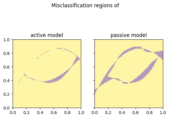
The passively trained model's prediction boundaries are not well-aligned with the ground truth, simply because there are fewer datapoints close to the ground truth boundaries, compared to the actively learned model. Datapoints far from the decision boundary contribute little to no information to the model. This results in a higher overall accuracy for the actively learned model.
print(f"Accuracy of actively trained model: {accuracies[-1] * 100:.1f}%")
print(f"Accuracy of passively trained model: {passive_acc * 100:.1f}%")

plt.plot(accuracies * 100, label="Active learning")
plt.hlines(
    y=passive_acc * 100,
    xmin=0,
    xmax=learning_rounds,
    linestyles="dashed",
    label="Passive baseline",
)
plt.xlabel("Active learning rounds")
plt.ylabel("Accuracy [%]")
plt.legend()
plt.show()
Accuracy of actively trained model: 97.2%
Accuracy of passively trained model: 92.1%
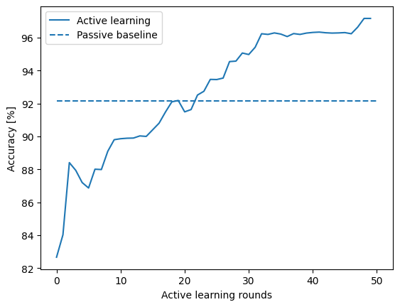
Here, the accuracy is plotted as a function of completed active learning rounds. The dashed line represents the accuracy of the passively trained model, with the same number of datapoints as the active one after the last iteration. One can see that the accuracy of the actively trained model is larger at the end, and that the point where the actively trained model surpasses the passively trained model is pretty early, meaning that less data is needed to achieve the same model quality.
This concludes the active learning tutorial for classification, where we have seen that active learning improves data efficiency by ensuring that datapoints are chosen closer to the decision boundary to maximize their informativeness about the true function.