Active Learning using Laplax¶

In this example notebook, we demonstrate how laplax can be used for active learning with a deep neural network. It is based on the article Information-Based Objective Functions for Active Data Selection by David MacKay.

Active learning means to pick the datapoints used for training iteratively and in a smart manner, maximizing the information they give about the network parameters. We start by implementing the four core mechanics necessary to do active learning: 1) Sample a target given an x-value from the true function 2) Train the model using a given dataset of points 3) Compute the posterior covariance of the model 4) Find the most informative datapoint using a heuristic based on the posterior covariance

Part 1) and 2) are identical to what you would do in passive learning, i.e. normally. Part 3) is where we are going to use laplax. For part 4), we are going to showcase the different heuristics introduced by MacKay.

Active learning then iterates through these steps in order to learn the function in a data-efficient manner. This is especially useful when labelling data is expensive, e.g. when it has to be labelled manually by experts or acquired through a physics experiment.

Reference: David J. C. MacKay, Information-Based Objective Functions for Active Data Selection, 1992

from copy import deepcopy
from functools import partial

import ipywidgets as widgets
import jax
import optax
from flax import nnx
from helper import DataLoader, Model, split, suppress_info_logging, train_model
from IPython.display import display
from jax import numpy as jnp
from jax import random, vmap
from matplotlib import pyplot as plt
from plotting import (
    ResultPlot,
    plot_model_comparison,
    show_animation,
)
from tqdm import tqdm

from laplax.curv import create_ggn_mv, create_posterior_fn
from laplax.eval import evaluate_for_given_prior_arguments
from laplax.eval.calibrate import optimize_prior_prec
from laplax.eval.metrics import nll_gaussian
from laplax.eval.pushforward import (
    lin_pred_mean,
    lin_pred_std,
    lin_setup,
    set_lin_pushforward,
    set_posterior_gp_kernel,
)

seed = 2392385
key = random.key(seed)

Problem setup¶

We first choose a function that we want to learn, for now a simple 1D to 1D function, the sinus cardinalis. We choose a one-dimensional problem for this example for ease of visualization, but everything is generalizable to more dimensions. First, we define a function that computes the value of the function at a given point, and adds Gaussian measurement noise.

This notebook uses a default noise variance of 0.01. When running the notebook interactively (e.g. in Jupyter or Colab) you can vary it with the slider below — there are more such controls further down. Remember to re-execute the cells beneath a widget after changing its value.

var_widget = widgets.FloatLogSlider(
    value=0.01, base=10, min=-3, max=0, step=0.001, description="Variance"
)
display(var_widget)

sample_variance = var_widget.value
print("Sample variance: ", sample_variance)


def sample_target(x, key, sample_variance=0.01):
    """Sample a target (label) for a given datapoint x.

    Args:
        x: x-value for which to sample a label
        key: PRNGKey to use for sampling
        sample_variance: Strength of added noise

    Returns:
        $y = f(x) + eps$ where $f$ is the sinc function
        and eps is Gaussian noise with mean zero and variance given by 'sample_variance'
    """
    x = x.squeeze()  # Assume one-dimensional x values
    y_true = jnp.sinc(x)
    noise = random.normal(key, y_true.shape) * jnp.sqrt(sample_variance)
    return y_true + noise


# Function without noise
def true_function(xs):
    key = random.key(seed)
    keys = random.split(key, len(xs))

    function = partial(sample_target, sample_variance=0.0)
    return vmap(function)(xs, keys)


# Initial dataset
x = jnp.concatenate((jnp.linspace(0.2, 2, 5), jnp.linspace(3.5, 5, 6)))[:, None]
n_initial_datapoints = x.shape[0]

keys = random.split(key, len(x))

sample = partial(sample_target, sample_variance=sample_variance)
y = vmap(sample)(x, keys)[:, None]

start_dataloader = DataLoader(x, y, batch_size=10)

Sample variance:  0.01

We now have a preliminary dataset of just eleven points, sampled from the function.

Model definition¶

Next, we define our deep neural network. Here, we use a network of 4 fully connected layers with a hidden dimension of 32.

@nnx.jit
def train_step(model, optimizer, x, y):
    def loss_fn(model):
        y_pred = model(x)
        return jnp.mean((y_pred - y) ** 2)

    loss, grads = nnx.value_and_grad(loss_fn)(model)
    optimizer.update(grads)

    return loss


start_model = Model(
    in_channels=1, hidden_channels=32, out_channels=1, rngs=nnx.Rngs(seed)
)

params = nnx.state(start_model)
total_params = sum(p.size for p in jax.tree.leaves(params))
print(f"Total number of parameters: {total_params}")

Total number of parameters: 2209

Training loop¶

We train our model on the small starting dataset, with MSE loss and optimizer adam.

lr = 5e-3
n_initial_epochs = start_dataloader.n_elements() * 100
optimizer = nnx.Optimizer(start_model, optax.adam(lr))
start_model = train_model(
    start_model, optimizer, start_dataloader, train_step, n_epochs=n_initial_epochs
)

[epoch 100]: loss: 0.0412


[epoch 200]: loss: 0.0208


[epoch 300]: loss: 0.0071


[epoch 400]: loss: 0.0009


[epoch 500]: loss: 0.0119


[epoch 600]: loss: 0.0000


[epoch 700]: loss: 0.0003


[epoch 800]: loss: 0.0030


[epoch 900]: loss: 0.0037


[epoch 1000]: loss: 0.0132


Final loss: 0.0316

Let's now visualize what we have so far:

# Trained model visualization
n_pred = 200
x_pred = jnp.linspace(0.0, 5.9, n_pred)[:, None]

y_true = true_function(x_pred)
y_pred = start_model(x_pred)

_, ax = plt.subplots(figsize=(10, 5))
ResultPlot(ax, x_pred, y_pred, y_true, start_dataloader)
plt.show()

png

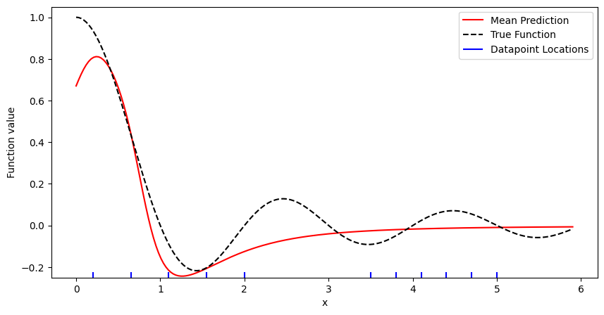
The plot visualizes the true function and the model's prediction. The markers on the x-axis visualize the location of the initial datapoints.

This concludes steps 1) and 2). Next, we turn to step 3), getting a posterior covariance kernel. This will give us the necessary information to make decisions about which datapoint to choose next.

The posterior covariance kernel is a function that takes two x-values and returns the estimated covariance between them given a (probabilistic) model. Since our deep neural network is not probabilistic, we need to add this probabilistic functionality. This is exactly what Laplax is designed to do. We use it to do a Laplace approximation in the weight space, which we push forward into the output space.

Uncertainty Estimation¶

Before computing the posterior, we choose how to approximate the curvature matrix.

By default, we choose the full curvature matrix. This is of course the most accurate, but most expensive option. Since our network is quite small, the full matrix would have only $2209^2 \text{ entries} \cdot 4 \text{ bytes} = 19.5 \text{ MB}$. Also, laplax never instantiates the full matrix, but performs the downstream calculations in a memory-efficient manner.

We use the full curvature by default. When running interactively, you can select one of the low-rank methods (lanczos, lobpcg) or the diagonal approximation in the dropdown below to see how this speeds up the computation.

lib_dropdown = widgets.Dropdown(
    options=["full", "diagonal", "lanczos", "lobpcg"],
    value="full",
    description="Curv. est.:",
)
display(lib_dropdown)

print(f"Curvature will be estimated using a {lib_dropdown.value} approximation.")
curv_type = lib_dropdown.value
low_rank_args = {
    "key": random.key(20),
    "rank": 50,
    "mv_jit": True,
}
curv_args = {} if curv_type in {"full", "diagonal"} else low_rank_args

Curvature will be estimated using a full approximation.

We start by implementing some functions that will ultimately yield the posterior covariance kernel computed from the model.

def get_posterior_fn(model, data):
    trainset = {"input": data.X, "target": data.y}
    model_fn, params = split(model)

    ggn_mv = create_ggn_mv(
        model_fn,
        params,
        trainset,
        loss_fn="mse",
    )

    return create_posterior_fn(
        curv_type=curv_type,
        mv=ggn_mv,
        layout=params,
        **curv_args,
    )


def get_posterior_covariance_kernel(model, posterior_fn, prior_prec):
    model_fn, params = split(model)
    gp_kernel, _ = set_posterior_gp_kernel(
        model_fn=model_fn,
        mean=params,
        posterior_fn=posterior_fn,
        prior_arguments={"prior_prec": prior_prec},
        dense=True,
        output_layout=1,
    )

    def vectorized_laplace_kernel(a, b):
        return jnp.vectorize(gp_kernel, signature="(d),(d)->(j,j)")(a, b)[..., 0]

    return vectorized_laplace_kernel

To compute the posterior kernel function, we need a prior precision. Lacking any domain knowledge, we just assume an uninformative prior (low precision). We are going to calibrate the prior precision in the next step anyway; this is just for a first visualization of the uncertainty.

prior_prec = 1e-4

posterior_fn = get_posterior_fn(start_model, start_dataloader)
kernel = get_posterior_covariance_kernel(start_model, posterior_fn, prior_prec)


# This cell executes near instantly, as no actual computation is performed yet.
# Everything is evaluated lazily.

By acquiring the kernel, we have essentially turned our deep neural network into a Gaussian process: The mean function is just the forward pass, and the covariance function is the kernel.

So let's visualize it like that! Thankfully, it is straight-forward to calculate the uncertainty from the kernel:

\[\text{std}(x) = \sqrt{k(x,x)}\]

There is a simpler way to get the model's uncertainty without using the full posterior kernel, by using the laplax.eval.pushforward.set_prob_predictive() function. We use the posterior kernel here, because we need its functionality for the other, more complex data acquisition rules.

def get_uncertainty_from_kernel(kernel, x_pred):
    result = kernel(x_pred, x_pred).squeeze()
    return jnp.sqrt(result)


uncertainty = get_uncertainty_from_kernel(kernel, x_pred)

_, ax = plt.subplots(figsize=(10, 5))
plot = ResultPlot(ax, x_pred, y_pred, y_true, start_dataloader)
plot.plot_uncertainty(uncertainty)
plot.finalize_plot()
plt.show()

png

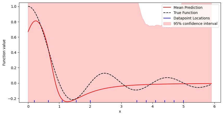
We see that the computed uncertainty is very large, going over the axis limit of the plot. Ideally, we would want it to be indicative of the standard deviation of the datapoints to the mean prediction: For a well-calibrated model, the residuals are Gaussian with a standard deviation that is equal to the model's uncertainty. Here however, the model is very underconfident.

To counter this, we calibrate the model on the data by tuning the prior precision. We do this by grid searching a range of precision values and evaluating a Gaussian negative log likelihood objective for the data points under the model uncertainty. This is also something laplax can do for us.

Prior precision calibration¶

def calibrate_prior_precision(data, model, posterior_fn, grid_params):
    """Calibrate the prior precision.

    Args:
        data: dataloader to use for calibration
        model: nnx.Module
        posterior_fn: posterior function of the model,
        precomputed by laplax
        grid_params: dict of parameters for grid search

    Returns:
        Calibrated prior precision.
    """
    calibration_batch = {"input": data.X, "target": data.y}
    model_fn, params = split(model)

    prob_predictive = partial(
        set_lin_pushforward,
        model_fn=model_fn,
        mean_params=params,
        posterior_fn=posterior_fn,
        pushforward_fns=[
            lin_setup,
            lin_pred_mean,
            lin_pred_std,
        ],
    )

    @jax.jit
    def nll_objective(prior_arguments, batch):
        return evaluate_for_given_prior_arguments(
            prior_arguments=prior_arguments,
            data=batch,
            set_prob_predictive=prob_predictive,
            metric=nll_gaussian,
        )

    # Optimize via grid search
    guess_magnitude = jnp.log10(grid_params["current_guess"])
    prior_prec = optimize_prior_prec(
        objective=partial(nll_objective, batch=calibration_batch),
        log_prior_prec_min=guess_magnitude - grid_params["magnitudes_to_search"] / 2.0,
        log_prior_prec_max=guess_magnitude + grid_params["magnitudes_to_search"] / 2.0,
        grid_size=grid_params["grid_size"],
    )
    return prior_prec


grid_params = {
    "current_guess": 100.0,  # / sample_variance,
    "magnitudes_to_search": 6,
    "grid_size": 50,
}

prior_prec = calibrate_prior_precision(
    start_dataloader, start_model, posterior_fn, grid_params
)

print("Prior precision: ", prior_prec)

[32m2026-06-16 09:34:25.845[0m | [1mINFO    [0m | [36mlaplax.eval.calibrate[0m:[36mgrid_search[0m:[36m110[0m - [1mTook 0.6266 seconds, prior prec: 0.1000, result: 0.116434[0m


[32m2026-06-16 09:34:26.114[0m | [1mINFO    [0m | [36mlaplax.eval.calibrate[0m:[36mgrid_search[0m:[36m110[0m - [1mTook 0.2678 seconds, prior prec: 0.1326, result: 0.101536[0m


[32m2026-06-16 09:34:26.385[0m | [1mINFO    [0m | [36mlaplax.eval.calibrate[0m:[36mgrid_search[0m:[36m110[0m - [1mTook 0.2710 seconds, prior prec: 0.1758, result: 0.086584[0m


[32m2026-06-16 09:34:26.648[0m | [1mINFO    [0m | [36mlaplax.eval.calibrate[0m:[36mgrid_search[0m:[36m110[0m - [1mTook 0.2614 seconds, prior prec: 0.2330, result: 0.071651[0m


[32m2026-06-16 09:34:26.915[0m | [1mINFO    [0m | [36mlaplax.eval.calibrate[0m:[36mgrid_search[0m:[36m110[0m - [1mTook 0.2666 seconds, prior prec: 0.3089, result: 0.056718[0m


[32m2026-06-16 09:34:27.179[0m | [1mINFO    [0m | [36mlaplax.eval.calibrate[0m:[36mgrid_search[0m:[36m110[0m - [1mTook 0.2636 seconds, prior prec: 0.4095, result: 0.041704[0m


[32m2026-06-16 09:34:27.448[0m | [1mINFO    [0m | [36mlaplax.eval.calibrate[0m:[36mgrid_search[0m:[36m110[0m - [1mTook 0.2673 seconds, prior prec: 0.5429, result: 0.026491[0m


[32m2026-06-16 09:34:27.704[0m | [1mINFO    [0m | [36mlaplax.eval.calibrate[0m:[36mgrid_search[0m:[36m110[0m - [1mTook 0.2553 seconds, prior prec: 0.7197, result: 0.010925[0m


[32m2026-06-16 09:34:27.976[0m | [1mINFO    [0m | [36mlaplax.eval.calibrate[0m:[36mgrid_search[0m:[36m110[0m - [1mTook 0.2717 seconds, prior prec: 0.9541, result: -0.005176[0m


[32m2026-06-16 09:34:28.244[0m | [1mINFO    [0m | [36mlaplax.eval.calibrate[0m:[36mgrid_search[0m:[36m110[0m - [1mTook 0.2673 seconds, prior prec: 1.2649, result: -0.022011[0m


[32m2026-06-16 09:34:28.503[0m | [1mINFO    [0m | [36mlaplax.eval.calibrate[0m:[36mgrid_search[0m:[36m110[0m - [1mTook 0.2584 seconds, prior prec: 1.6768, result: -0.039818[0m


[32m2026-06-16 09:34:28.759[0m | [1mINFO    [0m | [36mlaplax.eval.calibrate[0m:[36mgrid_search[0m:[36m110[0m - [1mTook 0.2549 seconds, prior prec: 2.2230, result: -0.058870[0m


[32m2026-06-16 09:34:29.031[0m | [1mINFO    [0m | [36mlaplax.eval.calibrate[0m:[36mgrid_search[0m:[36m110[0m - [1mTook 0.2714 seconds, prior prec: 2.9471, result: -0.079461[0m


[32m2026-06-16 09:34:29.290[0m | [1mINFO    [0m | [36mlaplax.eval.calibrate[0m:[36mgrid_search[0m:[36m110[0m - [1mTook 0.2578 seconds, prior prec: 3.9069, result: -0.101893[0m


[32m2026-06-16 09:34:29.552[0m | [1mINFO    [0m | [36mlaplax.eval.calibrate[0m:[36mgrid_search[0m:[36m110[0m - [1mTook 0.2617 seconds, prior prec: 5.1795, result: -0.126442[0m


[32m2026-06-16 09:34:29.816[0m | [1mINFO    [0m | [36mlaplax.eval.calibrate[0m:[36mgrid_search[0m:[36m110[0m - [1mTook 0.2630 seconds, prior prec: 6.8665, result: -0.153343[0m


[32m2026-06-16 09:34:30.080[0m | [1mINFO    [0m | [36mlaplax.eval.calibrate[0m:[36mgrid_search[0m:[36m110[0m - [1mTook 0.2634 seconds, prior prec: 9.1030, result: -0.182782[0m


[32m2026-06-16 09:34:30.350[0m | [1mINFO    [0m | [36mlaplax.eval.calibrate[0m:[36mgrid_search[0m:[36m110[0m - [1mTook 0.2695 seconds, prior prec: 12.0679, result: -0.214912[0m


[32m2026-06-16 09:34:30.612[0m | [1mINFO    [0m | [36mlaplax.eval.calibrate[0m:[36mgrid_search[0m:[36m110[0m - [1mTook 0.2604 seconds, prior prec: 15.9986, result: -0.249875[0m


[32m2026-06-16 09:34:30.873[0m | [1mINFO    [0m | [36mlaplax.eval.calibrate[0m:[36mgrid_search[0m:[36m110[0m - [1mTook 0.2605 seconds, prior prec: 21.2095, result: -0.287839[0m


[32m2026-06-16 09:34:31.149[0m | [1mINFO    [0m | [36mlaplax.eval.calibrate[0m:[36mgrid_search[0m:[36m110[0m - [1mTook 0.2751 seconds, prior prec: 28.1177, result: -0.329035[0m


[32m2026-06-16 09:34:31.426[0m | [1mINFO    [0m | [36mlaplax.eval.calibrate[0m:[36mgrid_search[0m:[36m110[0m - [1mTook 0.2761 seconds, prior prec: 37.2759, result: -0.373771[0m


[32m2026-06-16 09:34:31.688[0m | [1mINFO    [0m | [36mlaplax.eval.calibrate[0m:[36mgrid_search[0m:[36m110[0m - [1mTook 0.2610 seconds, prior prec: 49.4171, result: -0.422441[0m


[32m2026-06-16 09:34:31.955[0m | [1mINFO    [0m | [36mlaplax.eval.calibrate[0m:[36mgrid_search[0m:[36m110[0m - [1mTook 0.2659 seconds, prior prec: 65.5128, result: -0.475499[0m


[32m2026-06-16 09:34:32.219[0m | [1mINFO    [0m | [36mlaplax.eval.calibrate[0m:[36mgrid_search[0m:[36m110[0m - [1mTook 0.2637 seconds, prior prec: 86.8511, result: -0.533411[0m


[32m2026-06-16 09:34:32.483[0m | [1mINFO    [0m | [36mlaplax.eval.calibrate[0m:[36mgrid_search[0m:[36m110[0m - [1mTook 0.2626 seconds, prior prec: 115.1395, result: -0.596580[0m


[32m2026-06-16 09:34:32.754[0m | [1mINFO    [0m | [36mlaplax.eval.calibrate[0m:[36mgrid_search[0m:[36m110[0m - [1mTook 0.2707 seconds, prior prec: 152.6418, result: -0.665231[0m


[32m2026-06-16 09:34:33.023[0m | [1mINFO    [0m | [36mlaplax.eval.calibrate[0m:[36mgrid_search[0m:[36m110[0m - [1mTook 0.2678 seconds, prior prec: 202.3589, result: -0.739302[0m


[32m2026-06-16 09:34:33.274[0m | [1mINFO    [0m | [36mlaplax.eval.calibrate[0m:[36mgrid_search[0m:[36m110[0m - [1mTook 0.2510 seconds, prior prec: 268.2694, result: -0.818325[0m


[32m2026-06-16 09:34:33.528[0m | [1mINFO    [0m | [36mlaplax.eval.calibrate[0m:[36mgrid_search[0m:[36m110[0m - [1mTook 0.2530 seconds, prior prec: 355.6478, result: -0.901334[0m


[32m2026-06-16 09:34:33.799[0m | [1mINFO    [0m | [36mlaplax.eval.calibrate[0m:[36mgrid_search[0m:[36m110[0m - [1mTook 0.2706 seconds, prior prec: 471.4865, result: -0.986813[0m


[32m2026-06-16 09:34:34.091[0m | [1mINFO    [0m | [36mlaplax.eval.calibrate[0m:[36mgrid_search[0m:[36m110[0m - [1mTook 0.2906 seconds, prior prec: 625.0550, result: -1.072649[0m


[32m2026-06-16 09:34:34.360[0m | [1mINFO    [0m | [36mlaplax.eval.calibrate[0m:[36mgrid_search[0m:[36m110[0m - [1mTook 0.2680 seconds, prior prec: 828.6424, result: -1.156096[0m


[32m2026-06-16 09:34:34.615[0m | [1mINFO    [0m | [36mlaplax.eval.calibrate[0m:[36mgrid_search[0m:[36m110[0m - [1mTook 0.2544 seconds, prior prec: 1098.5405, result: -1.233691[0m


[32m2026-06-16 09:34:34.880[0m | [1mINFO    [0m | [36mlaplax.eval.calibrate[0m:[36mgrid_search[0m:[36m110[0m - [1mTook 0.2646 seconds, prior prec: 1456.3474, result: -1.301120[0m


[32m2026-06-16 09:34:35.145[0m | [1mINFO    [0m | [36mlaplax.eval.calibrate[0m:[36mgrid_search[0m:[36m110[0m - [1mTook 0.2645 seconds, prior prec: 1930.6971, result: -1.352986[0m


[32m2026-06-16 09:34:35.398[0m | [1mINFO    [0m | [36mlaplax.eval.calibrate[0m:[36mgrid_search[0m:[36m110[0m - [1mTook 0.2516 seconds, prior prec: 2559.5469, result: -1.382460[0m


[32m2026-06-16 09:34:35.663[0m | [1mINFO    [0m | [36mlaplax.eval.calibrate[0m:[36mgrid_search[0m:[36m110[0m - [1mTook 0.2650 seconds, prior prec: 3393.2197, result: -1.380809[0m


[32m2026-06-16 09:34:35.931[0m | [1mINFO    [0m | [36mlaplax.eval.calibrate[0m:[36mgrid_search[0m:[36m110[0m - [1mTook 0.2672 seconds, prior prec: 4498.4297, result: -1.336730[0m


[32m2026-06-16 09:34:36.182[0m | [1mINFO    [0m | [36mlaplax.eval.calibrate[0m:[36mgrid_search[0m:[36m110[0m - [1mTook 0.2505 seconds, prior prec: 5963.6182, result: -1.235484[0m


[32m2026-06-16 09:34:36.444[0m | [1mINFO    [0m | [36mlaplax.eval.calibrate[0m:[36mgrid_search[0m:[36m110[0m - [1mTook 0.2609 seconds, prior prec: 7906.0396, result: -1.057726[0m


[32m2026-06-16 09:34:36.708[0m | [1mINFO    [0m | [36mlaplax.eval.calibrate[0m:[36mgrid_search[0m:[36m110[0m - [1mTook 0.2631 seconds, prior prec: 10481.1309, result: -0.777971[0m


[32m2026-06-16 09:34:36.964[0m | [1mINFO    [0m | [36mlaplax.eval.calibrate[0m:[36mgrid_search[0m:[36m110[0m - [1mTook 0.2556 seconds, prior prec: 13894.9531, result: -0.362568[0m


[32m2026-06-16 09:34:37.229[0m | [1mINFO    [0m | [36mlaplax.eval.calibrate[0m:[36mgrid_search[0m:[36m110[0m - [1mTook 0.2642 seconds, prior prec: 18420.6934, result: 0.233001[0m


[32m2026-06-16 09:34:37.481[0m | [1mINFO    [0m | [36mlaplax.eval.calibrate[0m:[36mgrid_search[0m:[36m110[0m - [1mTook 0.2516 seconds, prior prec: 24420.5215, result: 1.067671[0m


[32m2026-06-16 09:34:37.742[0m | [1mINFO    [0m | [36mlaplax.eval.calibrate[0m:[36mgrid_search[0m:[36m110[0m - [1mTook 0.2595 seconds, prior prec: 32374.5566, result: 2.219514[0m


[32m2026-06-16 09:34:38.006[0m | [1mINFO    [0m | [36mlaplax.eval.calibrate[0m:[36mgrid_search[0m:[36m110[0m - [1mTook 0.2637 seconds, prior prec: 42919.3125, result: 3.791983[0m


[32m2026-06-16 09:34:38.276[0m | [1mINFO    [0m | [36mlaplax.eval.calibrate[0m:[36mgrid_search[0m:[36m110[0m - [1mTook 0.2694 seconds, prior prec: 56898.6133, result: 5.922196[0m


[32m2026-06-16 09:34:38.530[0m | [1mINFO    [0m | [36mlaplax.eval.calibrate[0m:[36mgrid_search[0m:[36m110[0m - [1mTook 0.2529 seconds, prior prec: 75431.1250, result: 8.791898[0m


[32m2026-06-16 09:34:38.793[0m | [1mINFO    [0m | [36mlaplax.eval.calibrate[0m:[36mgrid_search[0m:[36m110[0m - [1mTook 0.2623 seconds, prior prec: 100000.0000, result: 12.642029[0m


[32m2026-06-16 09:34:38.794[0m | [1mINFO    [0m | [36mlaplax.eval.calibrate[0m:[36mgrid_search[0m:[36m139[0m - [1mChosen prior prec = 2559.5469[0m


Prior precision:  2559.5469

We plot the learned network again, this time with the calibrated uncertainty.

y_mean = start_model(x_pred)
kernel = get_posterior_covariance_kernel(start_model, posterior_fn, prior_prec)
y_std = get_uncertainty_from_kernel(kernel, x_pred)

_, ax = plt.subplots(figsize=(10, 5))
plot = ResultPlot(ax, x_pred, y_pred, y_true, start_dataloader)
plot.plot_uncertainty(y_std)
plot.finalize_plot()
plt.show()

png

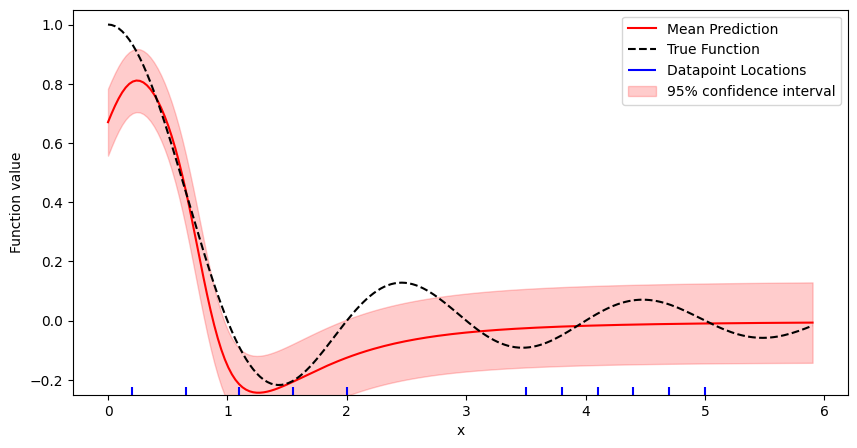
Now, the uncertainty resembles the magnitude of the error our model makes much better.

Note: We are calibrating the model's prior precision on the training set, which is not ideal. Instead, in practice, calibration should be performed on a holdout dataset. We are doing this for the sake of simplicity and because we are assuming that acquiring data is hard.

Maximizing total information gain¶

Now, let's get into how to use the obtained kernel for active learning, approaching step 4) of the active learning protocol.

The question we need to answer here is the following: Where do we need to sample next in order to maximize the information the learning algorithm gets about the parameters from the sampled point?

The answer is given by the total information gain criterion, formula 3.6 in the MacKay paper: $$\text{total information gain} = \frac{1}{2} \log\left(1 + \text{prior precision} \cdot \text{kernel}(x_\text{pred},x_\text{pred})\right) $$ As MacKay points out, the maximum of this criterion function is exactly at the maximum of the standard deviation we just plotted, as long as the prior variance is constant. This yields a nice interpretation: To maximize the information gain, sample where we are most uncertain.

It is important to note that calibration can actually influence the position of the maximum, as the prior precision influences the information criterion in a non-linear way.

def find_maximum(x_pred, criterion):
    """Find the point in x_pred where criterion is maximal.

    Args:
        x_pred: Array of x values of which uncertainty is known
        criterion: The criterion values to maximize

    Returns:
        x-value with largest criterion value
    """
    next_index = jnp.argmax(criterion)
    return x_pred[next_index]


def total_information_gain(kernel, prior_prec, x_pred):
    """Find point where the total information gain is maximal.

    Args:
        kernel: Posterior covariance kernel of the model
        prior_prec: Prior of measurement precision
        x_pred: Candidate points

    Returns:
        Total information gain criterion evaluated at x_pred.
    """
    variances_x = kernel(x_pred, x_pred)
    return jnp.log(1 + prior_prec * variances_x) / 2.0


next_datapoint = find_maximum(
    x_pred, total_information_gain(kernel, prior_prec, x_pred)
)

Active learning loop¶

Now that we have implemented and demonstrated all four steps, we can implement the full active learning loop, iteratively sampling the next datapoint, adding it to the trainset, continuing training for 100 epochs, recomputing the uncertainty, and finding the next best location. We also recalibrate the model in every step, as the calibration depends on the number of datapoints we have. We again calibrate by grid search, this time with a small grid around the previous value.

The active learning loop takes as one argument a criterion function. This function takes the kernel, prior precision and an array x_pred as arguments and outputs the information criterion values at the x_pred points. Our first such function is the total_information_gain, which we demonstrate here. For a returned criterion array, the active learning loop then finds the maximum and chooses this as next datapoint location.

epochs_per_learning_round = 100
learning_rounds = 16


def active_learning_loop(
    model,
    criterion_fn,
    next_datapoint,
    dataloader,
    prior_prec,
    learning_rounds,
    verbose_rounds=2,
):
    # To keep the rendered output readable, we only print the details of the
    # first `verbose_rounds` rounds (set verbose_rounds=learning_rounds to see
    # them all).
    key = random.key(21780)
    keys = random.split(key, learning_rounds)

    plot_data = []
    optimizer = nnx.Optimizer(model, optax.adam(lr))

    for i, key in tqdm(enumerate(keys)):
        verbose = i < verbose_rounds
        if verbose:
            print(f"Active learning round {i + 1}")
        # 1) Sample new datapoint
        next_target = sample_target(
            next_datapoint, key, sample_variance=sample_variance
        )
        dataloader = dataloader.add(next_datapoint, jnp.atleast_2d(next_target))

        # 2) Continue training
        model = train_model(
            model,
            optimizer,
            dataloader,
            train_step,
            n_epochs=epochs_per_learning_round,
            verbose=verbose,
        )

        # 3) Calibrate and compute uncertainty
        posterior_fn = get_posterior_fn(model, dataloader)
        grid_params = {
            "current_guess": prior_prec,
            "magnitudes_to_search": 0.5,
            "grid_size": 10,
        }
        prior_prec = calibrate_prior_precision(
            dataloader, model, posterior_fn, grid_params
        )
        if verbose:
            print(f"Calibrated precision: {prior_prec:.0f}")
        kernel = get_posterior_covariance_kernel(model, posterior_fn, prior_prec)

        # 4) Find next datapoint location
        criterion = criterion_fn(kernel, prior_prec, x_pred)
        next_datapoint = find_maximum(x_pred, criterion)

        # Plotting
        y_mean = model(x_pred)
        plot_data.append((
            x_pred,
            y_mean,
            y_true,
            dataloader,
            criterion,
            next_datapoint,
        ))
        if verbose:
            print("-----------------------")
        elif i == verbose_rounds:
            print(f"... (running {learning_rounds - verbose_rounds} more rounds) ...")

    return plot_data, model, dataloader


dataloader = deepcopy(start_dataloader)
model = deepcopy(start_model)
with suppress_info_logging("laplax.eval.calibrate"):
    plot_data, active_model, active_dataloader = active_learning_loop(
        model,
        total_information_gain,
        next_datapoint,
        dataloader,
        prior_prec,
        learning_rounds,
    )

0it [00:00, ?it/s]

Active learning round 1


Final loss: 0.0104


Calibrated precision: 2113

1it [00:05, 5.53s/it]

-----------------------
Active learning round 2


Final loss: 0.0087


Calibrated precision: 2909

2it [00:10, 5.44s/it]

-----------------------

3it [00:15, 5.16s/it]

... (running 14 more rounds) ...

4it [00:20, 5.03s/it]

5it [00:25, 5.03s/it]

6it [00:30, 5.04s/it]

7it [00:35, 5.07s/it]

8it [00:40, 5.09s/it]

9it [00:45, 5.07s/it]

10it [00:50, 5.05s/it]

11it [00:56, 5.10s/it]

12it [01:00, 5.02s/it]

13it [01:05, 5.01s/it]

14it [01:11, 5.04s/it]

15it [01:15, 5.00s/it]

16it [01:20, 4.99s/it]

16it [01:20, 5.06s/it]

show_animation(plot_data)

The active learning loop samples mostly in the range between 0 and 1, where the true function varies most strongly, making it harder to learn in this area. This leads to larger residuals between the mean prediction and the data, which in turn leads to a higher covariance estimate. The information criterion chooses points with large posterior covariance.

In short, this means that the active learning loop focuses on the area where there is most performance to be gained.

Comparison to passive learning¶

To see the difference active learning makes, we compare the learned model to one that is passively trained, i.e. one where the datapoints are not chosen smartly.

For a fair comparison, we train the passive model with the same number of datapoints and for the same overall number of epochs. Note however that in active learning, epochs are much smaller in the beginning. By default the passive datapoints are sampled randomly (uniform); when running interactively you can switch to deterministic equidistant spacing via the dropdown below.

sampling_dropdown = widgets.Dropdown(
    options=["Random Uniform", "Equidistant"],
    value="Random Uniform",
    description="Sampling:",
)
display(sampling_dropdown)

n_passive_datapoints = n_initial_datapoints + learning_rounds
n_passive_epochs = n_initial_epochs + learning_rounds * epochs_per_learning_round

# Sample x-values according to selection
sampling_type = sampling_dropdown.value
random_uniform = random.uniform(key, shape=n_passive_datapoints, minval=0, maxval=5.9)
equidistant = jnp.linspace(0.0, 5.9, n_passive_datapoints)
passive_xs = random_uniform if sampling_type == "Random Uniform" else equidistant
passive_xs = passive_xs[:, None]

# Sample y-values
keys = random.split(key, len(passive_xs))
passive_ys = vmap(sample)(passive_xs, keys)[:, None]

# Train model with sampled data
passive_dataloader = DataLoader(passive_xs, passive_ys, batch_size=10)
if passive_dataloader.n_elements() != active_dataloader.n_elements():
    print("Number of datapoints for active and passive learning do not match!")

passive_model = Model(
    in_channels=1, hidden_channels=32, out_channels=1, rngs=nnx.Rngs(seed)
)

passive_optimizer = nnx.Optimizer(passive_model, optax.adam(lr))
passive_model = train_model(
    passive_model,
    passive_optimizer,
    passive_dataloader,
    train_step,
    n_epochs=n_passive_epochs,
)

# Predict with passive model
y_pred_passive = passive_model(x_pred)

# Predict with active model
y_pred_active = active_model(x_pred)

# Plot
fig, ax = plt.subplots(figsize=(10, 5))
plot_model_comparison(
    ax, x_pred, y_true, y_pred_passive, y_pred_active, passive_dataloader
)
plt.show()

# Compute RMSE to exact function
passive_rmse = jnp.sqrt(jnp.mean((y_pred_passive - y_true) ** 2))
active_rmse = jnp.sqrt(jnp.mean((y_pred_active - y_true) ** 2))

print(f"RMSE of passive model to true function: {passive_rmse:.2f}")
print(f"RMSE of active model to true function: {active_rmse:.2f}")

[epoch 100]: loss: 0.0253


[epoch 200]: loss: 0.0087


[epoch 300]: loss: 0.0100


[epoch 400]: loss: 0.0053


[epoch 500]: loss: 0.0104


[epoch 600]: loss: 0.0062


[epoch 700]: loss: 0.0099


[epoch 800]: loss: 0.0120


[epoch 900]: loss: 0.0070


[epoch 1000]: loss: 0.0046


[epoch 1100]: loss: 0.0038


[epoch 1200]: loss: 0.0058


[epoch 1300]: loss: 0.0100


[epoch 1400]: loss: 0.0040


[epoch 1500]: loss: 0.0037


[epoch 1600]: loss: 0.0023


[epoch 1700]: loss: 0.0041


[epoch 1800]: loss: 0.0026


[epoch 1900]: loss: 0.0083


[epoch 2000]: loss: 0.0035


[epoch 2100]: loss: 0.0031


[epoch 2200]: loss: 0.0032


[epoch 2300]: loss: 0.0051


[epoch 2400]: loss: 0.0053


[epoch 2500]: loss: 0.0056


[epoch 2600]: loss: 0.0041


Final loss: 0.0036

png

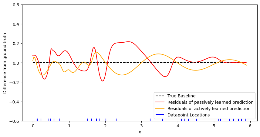
RMSE of passive model to true function: 0.41
RMSE of active model to true function: 0.39

The actively trained model is closer to the ground truth function especially in the area $x<1$. This leads to a slightly smaller RMSE.

Maximizing information about points of interest¶

We now implement the rule from chapter 4 of the MacKay paper as a criterion function. Here, we are interested in only a single point, about which we want to learn as much as possible. Formula 4.1 is given as: $$\text{marginal information gain} = -\frac{1}{2}\log\left(1 - \frac{\text{kernel} (x_\text{pred},x_\text{point})^2}{\text{kernel}(x_\text{point},x_\text{point}) (\text{prior precision}^{-1} + \text{kernel}(x_\text{pred},x_\text{pred}))}\right) $$

def information_gain_about_point(
    kernel, prior_prec, x_pred, point=0.0, no_sampling_zone=None
):
    """Calculate information gain about 'point' at 'x_pred'.

    Args:
        kernel: Posterior covariance kernel of the model
        prior_prec: Prior of measurement precision
        x_pred: Candidate points
        point: Point of interest where information should be maximized
        no_sampling_zone: Interval where prior precision is assumed to be extremely low,
            making information gain low in this region

    Returns:
        Information gain at x_pred values about the point of interest.
    """
    if no_sampling_zone is not None:
        no_sampling_xs = jnp.logical_and(
            x_pred > no_sampling_zone[0], x_pred < no_sampling_zone[1]
        )
        conditional_prior_prec = jnp.where(no_sampling_xs, 1e-10, prior_prec)
    else:
        conditional_prior_prec = prior_prec
    variance_u = kernel([point], [point])
    variance_nu = 1.0 / conditional_prior_prec
    variances_x = kernel(x_pred, x_pred)
    covariance_xu = kernel(x_pred, [point])
    return (
        -jnp.log(1 - covariance_xu**2 / (variance_u * (variance_nu + variances_x)))
        / 2.0
    )

interesting_point = 3.0
_information_gain_about_point = partial(
    information_gain_about_point, point=interesting_point
)

y_mean = start_model(x_pred)
kernel = get_posterior_covariance_kernel(start_model, posterior_fn, prior_prec)
criterion = _information_gain_about_point(kernel, prior_prec, x_pred)
next_datapoint = find_maximum(x_pred, criterion)

fig, ax = plt.subplots(figsize=(10, 5))
ax2 = ax.twinx()
plot = ResultPlot(
    (ax, ax2),
    x_pred,
    y_mean,
    y_true,
    start_dataloader,
    criterion,
    next_datapoint,
    [interesting_point],
)
plt.show()

png

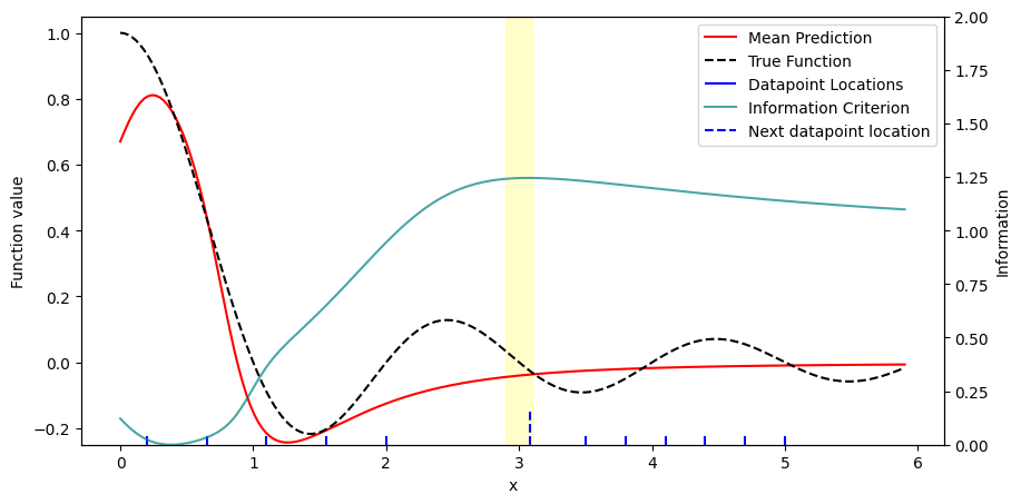
This verifies what is obvious: To maximize information gain about a point $x$, sample at point $x$. To make this more interesting, we can imagine an area around the interesting point, where we cannot sample for whatever reason. We can implement this by setting the prior precision in this region to a very small value. This tells the selection criterion that sampling in this area yields no information, and hence, the area will be avoided.

no_sampling_zone = (2.5, 3.5)
_information_gain_about_point = partial(
    _information_gain_about_point, no_sampling_zone=no_sampling_zone
)

dataloader = deepcopy(start_dataloader)
model = deepcopy(start_model)
with suppress_info_logging("laplax.eval.calibrate"):
    plot_data, _, _ = active_learning_loop(
        model,
        _information_gain_about_point,
        next_datapoint,
        dataloader,
        prior_prec,
        learning_rounds,
        verbose_rounds=0,
    )

0it [00:00, ?it/s]

1it [00:05, 5.69s/it]

... (running 16 more rounds) ...

2it [00:11, 5.64s/it]

3it [00:16, 5.54s/it]

4it [00:22, 5.52s/it]

5it [00:28, 5.63s/it]

6it [00:33, 5.71s/it]

7it [00:39, 5.72s/it]

8it [00:45, 5.75s/it]

9it [00:50, 5.67s/it]

10it [00:56, 5.72s/it]

11it [01:02, 5.63s/it]

12it [01:07, 5.59s/it]

13it [01:13, 5.62s/it]

14it [01:19, 5.62s/it]

15it [01:24, 5.65s/it]

16it [01:30, 5.65s/it]

idx_of_interesting_point = jnp.abs(x_pred - jnp.array(interesting_point)).argmin()
passive_mae = jnp.abs(
    y_pred_passive[idx_of_interesting_point] - y_true[idx_of_interesting_point]
).item()
active_mae = jnp.abs(
    y_mean[idx_of_interesting_point] - y_true[idx_of_interesting_point]
).item()

print(f"MAE of passive model to true function at interesting point: {passive_mae:.3f}")
print(f"MAE of active model to true function at interesting point: {active_mae:.3f}")

show_animation(plot_data, [interesting_point], no_sampling_zone)

MAE of passive model to true function at interesting point: 0.119
MAE of active model to true function at interesting point: 0.042

Here, it is important to consider in the evaluation that the passively trained model is the same as before, which can include datapoints from within the no-sampling zone. Still, the actively trained model outperforms the other one, simply because the training data is more relevant to the evaluated task.

Finally, we generalize the last criterion to apply to a set of interesting points. For simplicity, we assume that all points are equally interesting. Then, the mean marginal information gain from formula 4.4 is given as: $\(\text{mean marginal information gain} = \frac{1}{|\text{Points}|}\sum_\text{Points} \text{marginal information gain}(\text{point})$\)

def information_gain_about_points(
    kernel,
    prior_prec,
    x_pred,
    points,
):
    """Calculate information gain about 'points' at 'x_pred'.

    Args:
        kernel: Posterior covariance kernel of the model
        prior_prec: Prior of measurement precision
        x_pred: Candidate points
        points: Points of interest where information is sought

    Returns:
        Information gain at x_pred values about the points of interest.
    """
    single_point_information_gain = partial(
        information_gain_about_point, kernel, prior_prec, x_pred
    )
    single_criterions = jnp.vectorize(single_point_information_gain)(points)
    return jnp.mean(single_criterions.squeeze(-1), axis=0)

interesting_points = jnp.array([1.0, 3.5, 3.7])
criterion_fn = partial(information_gain_about_points, points=interesting_points)
criterion = criterion_fn(kernel, prior_prec, x_pred)
next_datapoint = find_maximum(x_pred, criterion)

dataloader = deepcopy(start_dataloader)
model = deepcopy(start_model)
with suppress_info_logging("laplax.eval.calibrate"):
    plot_data, _, _ = active_learning_loop(
        model,
        criterion_fn,
        next_datapoint,
        dataloader,
        prior_prec,
        learning_rounds,
        verbose_rounds=0,
    )

0it [00:00, ?it/s]

1it [00:05, 5.80s/it]

... (running 16 more rounds) ...

2it [00:11, 5.72s/it]

3it [00:17, 5.69s/it]

4it [00:22, 5.65s/it]

5it [00:28, 5.73s/it]

6it [00:34, 5.76s/it]

7it [00:40, 5.79s/it]

8it [00:46, 5.87s/it]

9it [00:52, 5.90s/it]

10it [00:58, 5.91s/it]

11it [01:03, 5.81s/it]

12it [01:09, 5.82s/it]

13it [01:15, 5.85s/it]

14it [01:21, 5.87s/it]

15it [01:27, 5.85s/it]

16it [01:33, 5.82s/it]

16it [01:33, 5.81s/it]

indices_of_points = jnp.abs(
    jnp.atleast_2d(x_pred) - jnp.atleast_2d(interesting_points)
).argmin(axis=0)

passive_rmse = jnp.sqrt(
    jnp.mean((y_pred_passive[indices_of_points] - y_true[indices_of_points]) ** 2)
).item()
active_rmse = jnp.sqrt(
    jnp.mean((y_mean[indices_of_points] - y_true[indices_of_points]) ** 2)
).item()

print(
    f"RMSE of passive model to true function at interesting points: {passive_rmse:.3f}"
)
print(f"RMSE of active model to true function at interesting points: {active_rmse:.3f}")

show_animation(plot_data, interesting_points)

RMSE of passive model to true function at interesting points: 0.144
RMSE of active model to true function at interesting points: 0.074

Once again, the observed behaviour is intuitive: The chosen points are close to the points of interest, in this case close to the area where two points of interest are located. This is also reflected in the lower RMSE of the active model at the interesting points.

Summary¶

In this tutorial, we have implemented and illustrated three information criteria for active learning: We can use the total information gain to improve on passive learning globally, when no region is of special interest. We can also maximize the information gain about a point of interest or an area of interest. The points chosen by the criteria are intuitive, sampling closely to the regions of interest. In these more specialized tasks, the advantages of active learning becomes apparent.

We have also seen how to use laplax for computing the posterior covariance, which is needed for these criteria, and how to calibrate the prior precision.